Plotting AWS Spot Prices in Slack
For the past year or so I have been using Amazon Web Services (AWS) and have consistently desired to have an easy way to find recent spot price trends.
For those unaware, AWS has a service called Elastic Compute Cloud (EC2) which allows you to rent compute resources at an hourly rate. Rates are generally broken into three types:
- On-Demand: As the name implies you can start an on-demand machine at any time, terminate it at any time, and only pay for the time that you use (rounded up to the nearest hour). This is convenient, buts also the most expensive option on AWS
- Reserved: This option allows you to purchase machine time for longer periods of time starting at 1 year. Prices tend to be far cheaper than on-demand with the drawback that you purchase time in large blocks. This is good if you are running an always on web server, but not ideal if you use AWS for burst computation over the span of a few hours then terminate the instance. An example of this would be for running machine learning models as part of research.
- Spot Instance: Lastly, AWS offers the capability to bid on available EC2 capacity. The benefit is that costs are often 5-10x less, but if the market price exceeds your spot bid your instance is terminated.
My day to day workflow for PhD research is something like
- Arrive to the lab and lookup recent spot prices on EC2’s spot bidding console.
- If spot prices seem stable then create a spot bid instance and treat it like an on-demand instance for the day.
- Throughout the day save my work using a combination of
scp,git, and Amazon S3.
I set out to make (1) automatic by fetching the spot prices for a list of instance types, plotting recent spot prices with Seaborn, sending this to Slack, and automating the process with Apache Airflow.
Fetching Spot Price Data
The first step is to fetch data to plot. The easiest way to do this is using the AWS CLI which is installable via pip install awscli. If you haven’t used the cli before you also need to run aws configure to setup your AWS credentials.
You can now use the describe-spot-price-history api to get the data in json. Below is the call to aws with a sample of the data.
$ aws ec2 describe-spot-price-history --instance-types r3.8xlarge | head -n 20
{
    "SpotPriceHistory": [
        {
            "Timestamp": "2016-09-03T20:57:40.000Z",
            "ProductDescription": "Linux/UNIX",
            "InstanceType": "r3.8xlarge",
            "SpotPrice": "0.501000",
            "AvailabilityZone": "us-west-1a"
        },
        {
            "Timestamp": "2016-09-03T20:57:40.000Z",
            "ProductDescription": "Linux/UNIX",
            "InstanceType": "r3.8xlarge",
            "SpotPrice": "0.394100",
            "AvailabilityZone": "us-west-1b"
        },
        {
            "Timestamp": "2016-09-03T20:57:39.000Z",
            "ProductDescription": "Windows",
            "InstanceType": "r3.8xlarge",
Its also possible to change the region from the one configured by aws configure by supplying --region. The other important options are --start-time and --end-time which control what time period to query data from. Having this data is great, but we now need to bring it into python. The easiest way to do this is use subprocess.run to execute the command, capture the standard out, then have the json module parse the output.
The initial function signature looks like:
import subprocess
from datetime import datetime
import json
import matplotlib
matplotlib.use('Agg')
import pandas as pd
import seaborn as sns
import matplotlib.pyplot as plt

def get_spot_price_data(instance_types, start_time=None, end_time=None, region=None):
    """
    Fetches the current spot price history for the given instances types and date range for the
    specified region. If the region is not specified then it falls back to the defaults set by the
    environment.
    :param instance_types: list(str), list of instances to get price for
    :param start_time: starting time
    :param end_time: ending time
    :param region: region string, if None defaults
    :return: json dataset with correctly formatted columns
    """
The next block of code shows building the command line arguments, and calling subprocess.run.
if region is not None:
    command = ['aws', '--region', region, 'ec2', 'describe-spot-price-history']
else:
    command = ['aws', 'ec2', 'describe-spot-price-history']
options = []

if len(instance_types) < 1:
    raise ValueError('Expected instance_types to have at least one instance type')

options.extend(['--instance-types'] + list(instance_types))

if start_time is not None:
    options.extend(['--start-time', start_time.strftime('%Y-%m-%dT%H:%M:%S')])

if end_time is not None:
    options.extend(['--end-time', end_time.strftime('%Y-%m-%dT%H:%M:%S')])

try:
    output = subprocess.run(
        command + options,
        check=True,
        stdout=subprocess.PIPE,
        stderr=subprocess.PIPE
    )
except Exception as e:
    print(e.stdout.decode('utf-8'))
    print(e.stderr.decode('utf-8'))
    raise
There isn’t anything fancy here. The only notable things are that we are using UTC time, and we are checking the subprocess.run call for errors. The next step is to parse this into json and convert data to the type they should be such as converting the spot price from string to float.
j = json.loads(output.stdout.decode('utf-8'))
data = j['SpotPriceHistory']
for r in data:
    r['SpotPrice'] = float(r['SpotPrice'])
    ts = datetime.strptime(r['Timestamp'], '%Y-%m-%dT%H:%M:%S.%fZ')
    r['DateTime'] = ts
    r['Timestamp'] = ts.timestamp()

return data
This last section of code finally converts the output from the aws ec2 command to json, and converts the relevant fields from strings to floats/dates.
Next we’re going to use pandas to convert the json data to a table. Lets take a glance at the data now.
def create_plot(json_data, output):
    all_data = pd.DataFrame(json_data)
In [1]: all_data = get_spot_price_data(['r3.8xlarge', 'c3.8xlarge'])
In [2]: all_data
Out[2]:
AvailabilityZone DateTime InstanceType ProductDescription SpotPrice Timestamp
0 us-west-1a 2016-09-03 21:19:00 c3.8xlarge Linux/UNIX 0.2845 1.472959e+09
1 us-west-1b 2016-09-03 21:19:00 c3.8xlarge Linux/UNIX 0.2842 1.472959e+09
2 us-west-1a 2016-09-03 21:18:33 c3.8xlarge Linux/UNIX 0.2846 1.472959e+09
3 us-west-1a 2016-09-03 21:18:06 c3.8xlarge Linux/UNIX 0.2853 1.472959e+09
4 us-west-1b 2016-09-03 21:17:40 r3.8xlarge Windows 0.9637 1.472959e+09
5 us-west-1b 2016-09-03 21:17:14 r3.8xlarge Windows 0.9638 1.472959e+09
6 us-west-1b 2016-09-03 21:17:13 r3.8xlarge Linux/UNIX 0.4023 1.472959e+09
7 us-west-1b 2016-09-03 21:17:11 c3.8xlarge Linux/UNIX 0.2844 1.472959e+09
8 us-west-1b 2016-09-03 21:16:45 r3.8xlarge Windows 0.9637 1.472959e+09
9 us-west-1b 2016-09-03 21:16:44 c3.8xlarge Linux/UNIX 0.2845 1.472959e+09
10 us-west-1b 2016-09-03 21:16:18 r3.8xlarge Linux/UNIX 0.4085 1.472959e+09
11 us-west-1b 2016-09-03 21:16:16 c3.8xlarge Linux/UNIX 0.2843 1.472959e+09
12 us-west-1a 2016-09-03 21:14:54 c3.8xlarge Linux/UNIX 0.2855 1.472959e+09
13 us-west-1b 2016-09-03 21:14:30 r3.8xlarge Linux/UNIX 0.4003 1.472959e+09
14 us-west-1b 2016-09-03 21:14:30 r3.8xlarge Windows 0.9636 1.472959e+09
15 us-west-1a 2016-09-03 21:14:28 c3.8xlarge Linux/UNIX 0.2846 1.472959e+09
16 us-west-1b 2016-09-03 21:14:00 c3.8xlarge Linux/UNIX 0.2842 1.472959e+09
17 us-west-1b 2016-09-03 21:12:41 r3.8xlarge Windows 0.9637 1.472959e+09
18 us-west-1b 2016-09-03 21:12:39 c3.8xlarge Linux/UNIX 0.2841 1.472959e+09
19 us-west-1b 2016-09-03 21:12:14 r3.8xlarge Linux/UNIX 0.4023 1.472959e+09
20 us-west-1b 2016-09-03 21:11:47 r3.8xlarge Windows 0.9636 1.472959e+09
21 us-west-1b 2016-09-03 21:11:21 r3.8xlarge Linux/UNIX 0.3941 1.472959e+09
22 us-west-1b 2016-09-03 21:11:17 c3.8xlarge Linux/UNIX 0.2838 1.472959e+09
23 us-west-1b 2016-09-03 21:09:55 c3.8xlarge Linux/UNIX 0.2840 1.472959e+09
24 us-west-1b 2016-09-03 21:09:31 r3.8xlarge Windows 0.9635 1.472959e+09
25 us-west-1b 2016-09-03 21:09:04 r3.8xlarge Linux/UNIX 0.3861 1.472959e+09
26 us-west-1b 2016-09-03 21:08:05 c3.8xlarge Linux/UNIX 0.2841 1.472958e+09
27 us-west-1a 2016-09-03 21:06:20 r3.8xlarge Linux/UNIX 0.5010 1.472958e+09
28 us-west-1a 2016-09-03 21:06:19 r3.8xlarge Windows 0.9823 1.472958e+09
29 us-west-1a 2016-09-03 21:06:16 c3.8xlarge Linux/UNIX 0.2843 1.472958e+09There are a few things to notice that will be important for plotting. First, we should cut down to only listing prices for Linux/UNIX servers since at least for my use case I am not running Windows servers. Second, we’ll make sure that each row is unique when keyed by availability zone, instance type, and date time by dropping any duplicates. Both of these are easily done in pandas.
df = all_data[all_data['ProductDescription'] == 'Linux/UNIX']
df = df.drop_duplicates(subset=['DateTime', 'AvailabilityZone', 'InstanceType'])
The next bit of code I arrived at after finding that my original plots weren’t padded correctly. This is easily fixed by fetching the minimal and maximal dates to compute border padding width.
x_min = df['DateTime'].min()
x_max = df['DateTime'].max()
border_pad = (x_max - x_min) * 5 / 100
Finally, we are ready to plot the data using seaborn and matplotlib. The most useful plot would show a scatter plot of time versus spot price for each combination of instance type and availability zone. The easiest way to do this is use seaborn.FacetGrid with matplotlib.pyplot.scatter. Lets see the code then explain.
g = sns.FacetGrid(
    df,
    col='InstanceType',
    hue='AvailabilityZone',
    xlim=(x_min - border_pad, x_max + border_pad),
    legend_out=True,
    size=10,
    palette="Set1"
)
g.map(plt.scatter, 'DateTime', 'SpotPrice', s=4).add_legend()
plt.subplots_adjust(top=.9)
g.fig.suptitle('AWS Spot Prices between {start} and {end}'.format(start=x_min, end=x_max))
g.savefig(output, format='png')
The easiest way to understand how FacetGrid works is to first look at what we want each subplot made by plt.scatter to show. If we were using only using matplotlib, we might write something like plt.scatter(df['DateTime'], df['SpotPrice']). There are two issues with this though. First, plt.scatter can’t take a date so we would need to pass Timestamp which doesn’t format on labels as well by default. Second, this would pass all the data, and we want to partition by different variables (analogously facets) such as availability zone and instance type.
Seaborn makes this much easier by taking as input the entire dataframe with specifications of which columns to cut the data on as col, row, and hue. In our case we want separate plots for each instance so we use col for that. We plot the availability zone as hue so that it shows on the same plot, but with a different color.
The g.map call takes as argument the main plotting function (in this case plt.scatter) and the other arguments are used to determine which columns to plot. The final result looks like this after changing the date range to cover the past week. For the curious, plots are included for both us-west-1 and us-east-1
US West 1
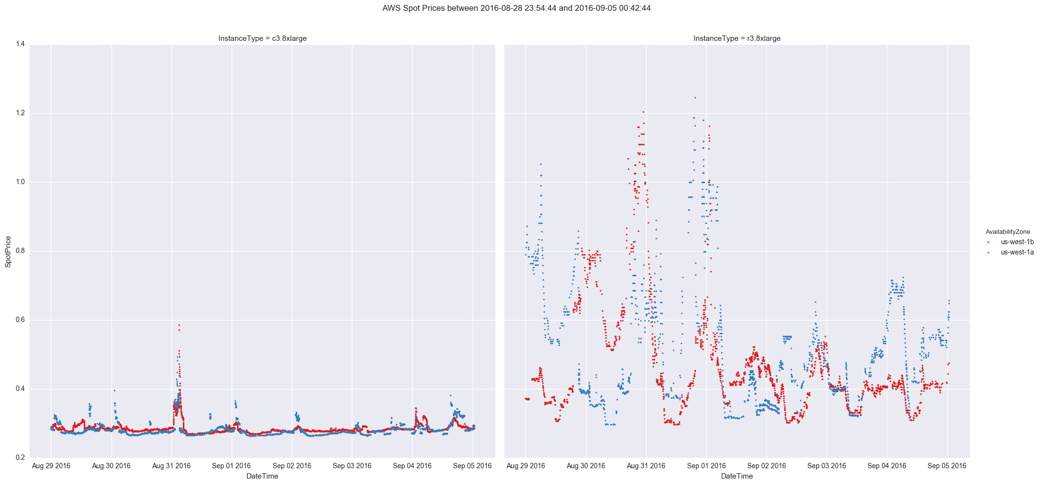
US East 1
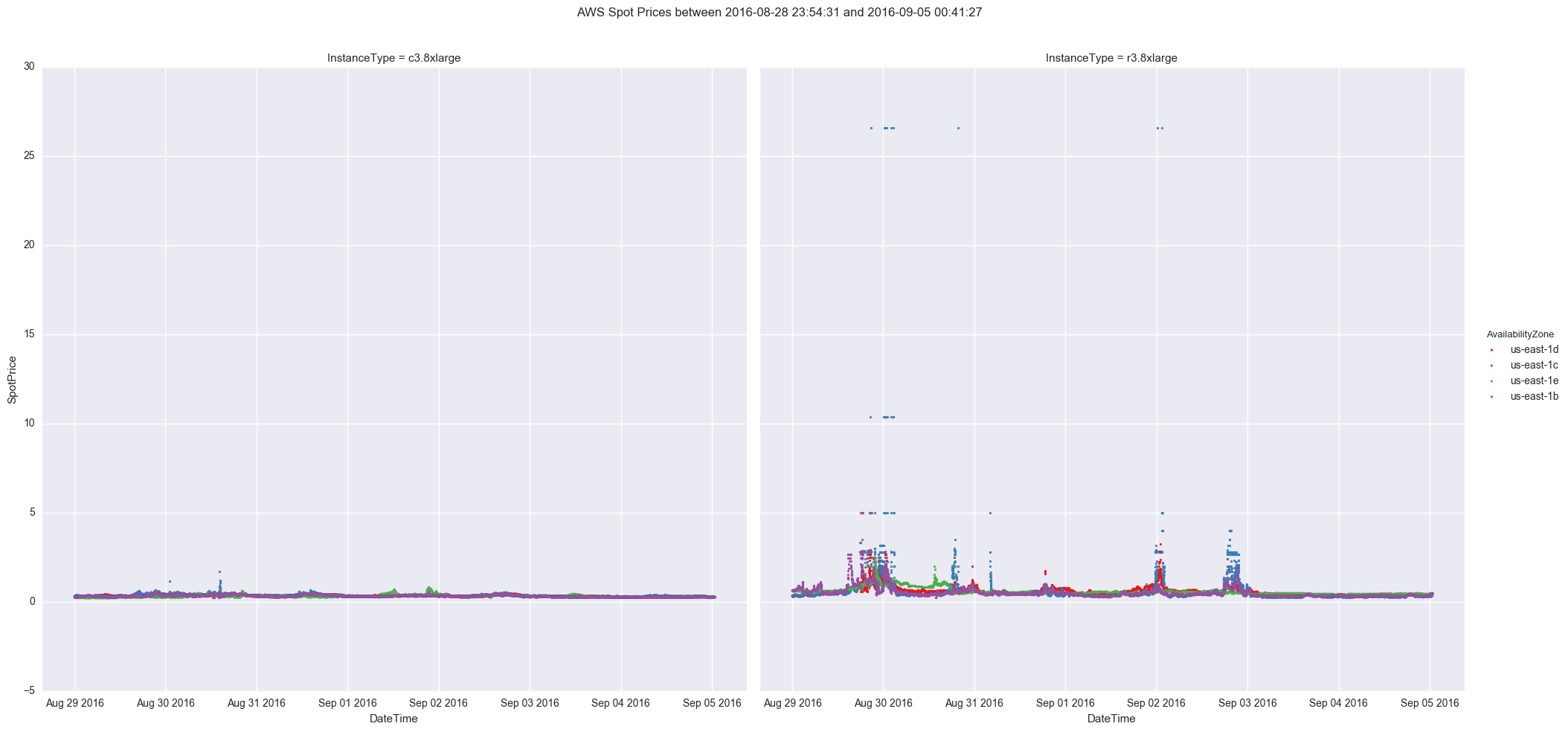
Certainly looks like us-east-1 is much more volatile for spot bidding which makes sense since it is also one of the oldest AWS regions. Lets move on to sending these plots to Slack.
There are quite a few Slack APIs around, but I found that slacker works quite well.
Once the plot is generated and saved its fairly easy to have slacker send a message and file to a specified channel.
import os
from slacker import Slacker

SLACK_API_TOKEN = os.environ.get('SLACK_API_TOKEN')
SLACK_CHANNEL = os.getenv('SLACK_CHANNEL', '#aws')


def notify(daily_file, weekly_file, stop_time, slack_api_token=None):
    if slack_api_token is None:
        slack_api_token = SLACK_API_TOKEN
    slack = Slacker(slack_api_token)
    slack.files.upload(
        daily_file, channels=[SLACK_CHANNEL],
        title='Daily AWS Spot Price ending on {}'.format(stop_time)
    )
    slack.files.upload(
        weekly_file, channels=[SLACK_CHANNEL],
        title='Weekly AWS Spot Price ending on {}'.format(stop_time)
    )
    slack.chat.post_message(
        '#aws', 'AWS Spot prices ending on {} are available'.format(stop_time),
        username='AWS Bot')
The slacker api makes things fairly simple here. Slack’s API token is stored in an environment variable along with the channel to post to. daily_file and weekly_file refer to plots made where the time periods spanned a day and a week. The code will upload the two files then inform the channel that the most recent spot price plots have been uploaded.
The last remaining tasks to wrap this up is creating a CLI to stitch everything together, and an Apache Airflow dag to run everything periodically.
By far the best python tool I’ve seen so far for making CLIs in python is Click.
The click API is fairly simple, poweful, and extensible. The relevant parts for this tutorial are:
- Click is decorator based which leaves the parameter list clean. It starts with using
click.command() click.optiontakes as arguments the name of the option and converts it to a variable name. The behavior is also configurable.click.argumenttakes the name of arguments which are represented as positional arguments
Now without further ado the code that stiches all these pieces together
from datetime import datetime
from datetime import timedelta
import os
from os import path
import click
from spot_reporter import reporting, slack


@click.command()
@click.option('--action', '-a', multiple=True, type=click.Choice(['email', 'slack']),
              help='Determine if/how to send aws pricing report')
@click.option('--output-dir', type=str, default='/tmp/spot-reporter',
              help='What directory to output files to, by default /tmp/spot-reporter')
@click.option('--end-time', type=str, default=None, help='Last time to check spot price for')
@click.option('--region', type=str, default=None,
              help='AWS region, by default uses the environment')
@click.option('--skip-generation', is_flag=True, help='Skip file generation')
@click.option('--slack-api-token', default=None,
              help='Slack API token, defaults to environment variable SLACK_API_TOKEN')
@click.argument('instance_types', nargs=-1, required=True)
def cli(action, output_dir, end_time, region, skip_generation, slack_api_token, instance_types):
    print('Running spot price reporter')
    daily_path = path.join(output_dir, 'aws_spot_price_daily.png')
    weekly_path = path.join(output_dir, 'aws_spot_price_weekly.png')
    if end_time is None:
        stop_datetime = datetime.now()
    else:
        stop_datetime = datetime.strptime(end_time, '%Y-%m-%dT%H:%M:%S')
    if not skip_generation:
        print('Getting AWS data')
        daily_data = reporting.get_spot_price_data(
            instance_types,
            start_time=stop_datetime - timedelta(days=1),
            end_time=stop_datetime,
            region=region
        )
        weekly_data = reporting.get_spot_price_data(
            instance_types,
            start_time=stop_datetime - timedelta(days=7),
            end_time=stop_datetime,
            region=region
        )

        if not path.exists(output_dir):
            os.makedirs(output_dir)

        print('Creating plots')
        reporting.create_plot(daily_data, daily_path)
        reporting.create_plot(weekly_data, weekly_path)

    if 'slack' in action:
        print('Uploading and messaging slack')
        slack.notify(daily_path, weekly_path, stop_datetime, slack_api_token=slack_api_token,
                     use_channel_time=use_channel_time)
Going from the top, this is what the code does:
- Determine where to store the images. Since we will send them over slack putting them in
/tmpseems appropriate since we don’t care if they are deleted afterwards. - Check and parse start and end datetimes.
- Fetch the data necesary for the daily and weekly report plots
- Create the output directory if it doesn’t exist
- Create the plots of daily and weekly spot price
- Send both of these over slack
The last step to automate this completely is to run it on a schedule. I chose to run it as an Apache Airflow DAG using the code below:
from airflow import DAG
from airflow.operators.bash_operator import BashOperator
from datetime import datetime, timedelta


default_args = {
    'owner': 'airflow',
    'depends_on_past': False,
    'start_date': datetime(2016, 8, 22),
    'retries': 1,
    'retry_delay': timedelta(minutes=1),
    }

dag = DAG('aws_spot_price_history', default_args=default_args, schedule_interval='@hourly')

run_all = BashOperator(
    task_id='run_all',
    bash_command='aws_spot_price_history --end-time {{ (execution_date + macros.timedelta(hours=1)).isoformat() }} --action slack --output-dir /tmp/spot-reporter/{{ (execution_date + macros.timedelta(hours=1)).isoformat() }} r3.8xlarge',
    dag=dag
)
Overall, this post covered a ton of ground and many tools, but I hope it can help you in either checking spot prices or seeing a way of automating useful tasks. All the code above is an installable python package at github.com/EntilZha/spot-price-reporter